Getting started with OnionNet#
OnionNet is a wrapper around graph-tool, targeted towards large multilayered networks. This tutorial will show you how to get started.
[ ]:
import sys
import os
import pandas as pd

import onionnet
print("onionnet package located at:", onionnet.__file__)
from onionnet import OnionNet
import onionnet.visualisation
import onionnet.exporter


import graph_tool.all as gt
from graph_tool.all import graph_draw

from onionnet.analytics import layer_stats, plot_layer_metagraph
onionnet package located at: /Users/agjanyunlu/Documents/Metabolomics/onionnet/onionnet/__init__.py
Inspecting data#
For this example we will use a network from Netzschleuder, which is loadable via graph-tool.
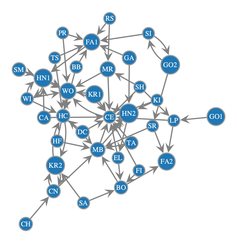
The data originates from a 1934 survey of school children in different grades, which was one of the earliest known uses of networks in sociology. For each child, they chose up to two students that they would like to sit next to in class.
The full dataset is from: grandjeanmartin/sociograms. Full citation can be found on Netzschleuder (https://networks.skewed.de/net/moreno_sociograms) and in the local markdown file (/.data/example_moreno_sociograms/About.md).
[2]:
g1 = gt.collection.ns["moreno_sociograms/grade_1"]
# pos_sfdp1 = gt.sfdp_layout(g)
g1
[2]:
<Graph object, directed, with 35 vertices and 67 edges, 2 internal vertex properties, 6 internal graph properties, at 0x104cf8d10>
[3]:
g2 = gt.collection.ns["moreno_sociograms/grade_2"]
# pos_sfdp2 = gt.sfdp_layout(g)
g2
[3]:
<Graph object, directed, with 29 vertices and 59 edges, 2 internal vertex properties, 6 internal graph properties, at 0x104cf98b0>
[4]:
graph_draw(g1, pos=g1.vp['_pos'], output_size=(400, 400))
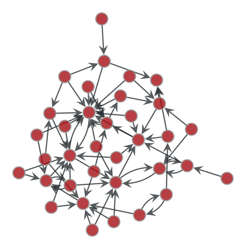
[4]:
<VertexPropertyMap object with value type 'vector<double>', for Graph 0x104cf8d10, at 0x161d62600>
[5]:
graph_draw(g2, pos=g2.vp['_pos'], output_size=(400, 400))
[5]:
<VertexPropertyMap object with value type 'vector<double>', for Graph 0x104cf98b0, at 0x161d634d0>
[6]:
list(g1.properties)
[6]:
[('v', 'name'),
 ('v', '_pos'),
 ('g', 'name'),
 ('g', 'description'),
 ('g', 'citation'),
 ('g', 'url'),
 ('g', 'upstream_license'),
 ('g', 'tags')]
However the basis of OnionNet is to read data in through pandas dataframes. So we do that here now to recreate the above graph. We will also rename the columns while we’re at it.
Creating an OnionNet object using pandas dfs#
Here we create a helper function to parse the data from the individual node or edge dataframes.
[7]:
def get_school_data(edges_or_nodes, grade, convert_to_str=False):
    if edges_or_nodes=='edges':
        df = pd.read_csv(f'.data/example_moreno_sociograms/grade_{grade}/edges.csv', sep=',', header=0)
        df.columns = ['source_id', 'target_id']
    elif edges_or_nodes=='nodes':
        df = pd.read_csv(f'.data/example_moreno_sociograms/grade_{grade}/nodes.csv', sep=',', header=0)
        df.columns = ['node_id', 'name', '_pos']
    else:
        raise ValueError("edges_or_nodes must be 'edges' or 'nodes', and a valid grade must be provided")
    # Here we will also convert all values to string
    if convert_to_str:
        for col in df.columns:
            df[col] = df[col].astype(str)
    return df
[8]:
print(get_school_data('nodes', 1).shape)
get_school_data('nodes', 1).head(10)
(35, 3)
[8]:
| node_id | name | _pos | |
|---|---|---|---|
| 0 | 0 | GO1 | array([-2.98488506, 0.86791962]) |
| 1 | 1 | LP | array([-2.95675841, 1.34825587]) |
| 2 | 2 | PR | array([-3.55699067, 3.00557276]) |
| 3 | 3 | WO | array([-3.34686456, 2.41781597]) |
| 4 | 4 | FA1 | array([-3.19714822, 2.96207321]) |
| 5 | 5 | CA | array([-3.72010476, 2.18584599]) |
| 6 | 6 | CE | array([-3.1286156 , 1.92922718]) |
| 7 | 7 | HN1 | array([-3.61538221, 2.70444297]) |
| 8 | 8 | FA2 | array([-2.36291912, 1.56251772]) |
| 9 | 9 | FI | array([-2.66954048, 1.51927661]) |
Now let’s say we want to create a multilayered network with the different classes from the school. To do this we will need to concatenate the dataframes.
[9]:
NUM_GRADES = 2
[10]:
df_nodes = pd.concat([get_school_data('nodes', i).assign(
    layer=f'grade_{i}')
    for i in range(1, NUM_GRADES+1)], ignore_index=True)
df_nodes
[10]:
| node_id | name | _pos | layer | |
|---|---|---|---|---|
| 0 | 0 | GO1 | array([-2.98488506, 0.86791962]) | grade_1 |
| 1 | 1 | LP | array([-2.95675841, 1.34825587]) | grade_1 |
| 2 | 2 | PR | array([-3.55699067, 3.00557276]) | grade_1 |
| 3 | 3 | WO | array([-3.34686456, 2.41781597]) | grade_1 |
| 4 | 4 | FA1 | array([-3.19714822, 2.96207321]) | grade_1 |
| ... | ... | ... | ... | ... |
| 59 | 24 | SH | array([ 1.60443291, -15.45916702]) | grade_2 |
| 60 | 25 | HF | array([ 1.50660581, -15.28444862]) | grade_2 |
| 61 | 26 | FS | array([ 1.4128519 , -15.46739683]) | grade_2 |
| 62 | 27 | AT | array([ 1.83319756, -15.69773967]) | grade_2 |
| 63 | 28 | MG | array([ 1.91520903, -15.22439855]) | grade_2 |
64 rows × 4 columns
[11]:
df_edges = pd.concat([get_school_data('edges', i).assign(
    source_layer=f'grade_{i}',
    target_layer=f'grade_{i}',
    interlayer=False)
    for i in range(1, NUM_GRADES+1)], ignore_index=True)
df_edges
[11]:
| source_id | target_id | source_layer | target_layer | interlayer | |
|---|---|---|---|---|---|
| 0 | 0 | 1 | grade_1 | grade_1 | False |
| 1 | 1 | 8 | grade_1 | grade_1 | False |
| 2 | 1 | 6 | grade_1 | grade_1 | False |
| 3 | 2 | 3 | grade_1 | grade_1 | False |
| 4 | 2 | 4 | grade_1 | grade_1 | False |
| ... | ... | ... | ... | ... | ... |
| 121 | 26 | 20 | grade_2 | grade_2 | False |
| 122 | 27 | 5 | grade_2 | grade_2 | False |
| 123 | 27 | 17 | grade_2 | grade_2 | False |
| 124 | 28 | 9 | grade_2 | grade_2 | False |
| 125 | 28 | 5 | grade_2 | grade_2 | False |
126 rows × 5 columns
From this we can create an OnionNet graph
[12]:
onion1 = OnionNet()

onion1.grow_onion(df_nodes=df_nodes,
           df_edges=df_edges,
           node_prop_cols=df_nodes.columns.to_list(),
           edge_prop_cols=df_edges.columns.to_list(),
           drop_na=True,
           drop_duplicates=True)
Nodes: in=64, dropped_na=0, deduped=0 → final=64
Edges: in=126, dropped_invalid=0, deduped=0 → final=126
To get a consistent layout for the graph we can use:
pos_sfdp = gt.sfdp_layout(onion1.core.graph)
Which will give us a standardised force-directed layout for the session and for this graph. But it will not be saved for the next session unless we do this with OnionNet, or generate it on the fly and save. In this tutorial we will load a pre-computed sfdp layout.
Beware however that this sfdp layout will be specific to your input dataframes and network. If you change the network or the input data for it, your ``node_id_hash`` or ``layer_hash`` will likely change.
[13]:
pos_sfdp = onionnet.visualisation.load_or_compute_layout(onion1.core.graph, filename='.getting_started_graph1_pos.tsv', override=False)
[load] Loaded layout for 64 rows from .getting_started_graph1_pos.tsv
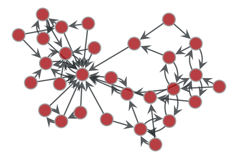
[14]:
graph_draw(onion1.core.graph, pos=pos_sfdp, output_size=(400, 400))
[14]:
<VertexPropertyMap object with value type 'vector<double>', for Graph 0x161d89d30, at 0x161dc08c0>
This is nice to see we have both our layers (i.e. grades) in the network. But it’s also clear to see they’re disconnected. Let’s simulate a scenario where some students in each grade are friends or siblings with those from other grades.
Multiple layers with interlayer connections#
[15]:
import numpy as np
import pandas as pd

def add_random_interlayer_edges(df_nodes, df_edges, num_interlayer_edges=10, seed=42):
    """
    Add random interlayer edges to an existing edges DataFrame.

    Parameters:
    - df_nodes: DataFrame containing nodes with at least 'id' and 'grade' columns.
    - df_edges: Existing edges DataFrame.
    - num_interlayer_edges: Number of random interlayer edges to create.
    - seed: Random seed for reproducibility.

    Returns:
    - Updated df_edges with added interlayer edges.
    """
    np.random.seed(seed)

    # Get unique grades from the nodes DataFrame.
    grades = df_nodes['layer'].unique()
    random_edges = []

    for _ in range(num_interlayer_edges):
        # Randomly select two different grades.
        source_grade, target_grade = np.random.choice(grades, size=2, replace=False)

        # Get nodes corresponding to each grade.
        source_nodes = df_nodes[df_nodes['layer'] == source_grade]
        target_nodes = df_nodes[df_nodes['layer'] == target_grade]

        # If one of the grades doesn't have any nodes, skip this iteration.
        if source_nodes.empty or target_nodes.empty:
            continue

        # Randomly select one node from each grade (assumes 'id' column exists).
        source_node = source_nodes.sample(n=1).iloc[0]['node_id']
        target_node = target_nodes.sample(n=1).iloc[0]['node_id']

        # Append a new interlayer edge.
        random_edges.append({
            'source_id': source_node,
            'target_id': target_node,
            'source_layer': source_grade,
            'target_layer': target_grade,
            'interlayer': True
        })

    # Convert the list of random edges into a DataFrame.
    df_random_edges = pd.DataFrame(random_edges)

    # Concatenate the random interlayer edges with the existing edges.
    updated_df_edges = pd.concat([df_edges, df_random_edges], ignore_index=True)

    return updated_df_edges

# Now add random interlayer edges.
df_edges_with_friends = add_random_interlayer_edges(df_nodes, df_edges, num_interlayer_edges=10, seed=42)
df_edges_with_friends
[15]:
| source_id | target_id | source_layer | target_layer | interlayer | |
|---|---|---|---|---|---|
| 0 | 0 | 1 | grade_1 | grade_1 | False |
| 1 | 1 | 8 | grade_1 | grade_1 | False |
| 2 | 1 | 6 | grade_1 | grade_1 | False |
| 3 | 2 | 3 | grade_1 | grade_1 | False |
| 4 | 2 | 4 | grade_1 | grade_1 | False |
| ... | ... | ... | ... | ... | ... |
| 131 | 17 | 17 | grade_2 | grade_1 | True |
| 132 | 4 | 15 | grade_1 | grade_2 | True |
| 133 | 9 | 10 | grade_1 | grade_2 | True |
| 134 | 14 | 26 | grade_2 | grade_1 | True |
| 135 | 10 | 23 | grade_1 | grade_2 | True |
136 rows × 5 columns
[16]:
onion2 = OnionNet()

onion2.grow_onion(df_nodes=df_nodes,
           df_edges=df_edges_with_friends,
           node_prop_cols=df_nodes.columns.to_list(),
           edge_prop_cols=df_edges_with_friends.columns.to_list(),
           drop_na=False,
           drop_duplicates=False)
Nodes: in=64, dropped_na=0, deduped=0 → final=64
Edges: in=136, dropped_invalid=0, deduped=0 → final=136
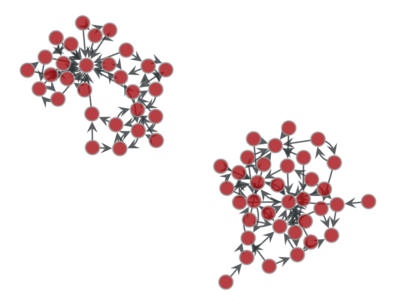
[17]:
graph_draw(onion2.core.graph, pos=pos_sfdp, output_size=(400, 400))
[17]:
<VertexPropertyMap object with value type 'vector<double>', for Graph 0x161d8ac30, at 0x161dc1160>
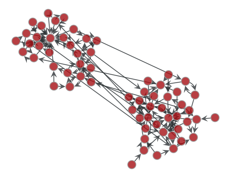
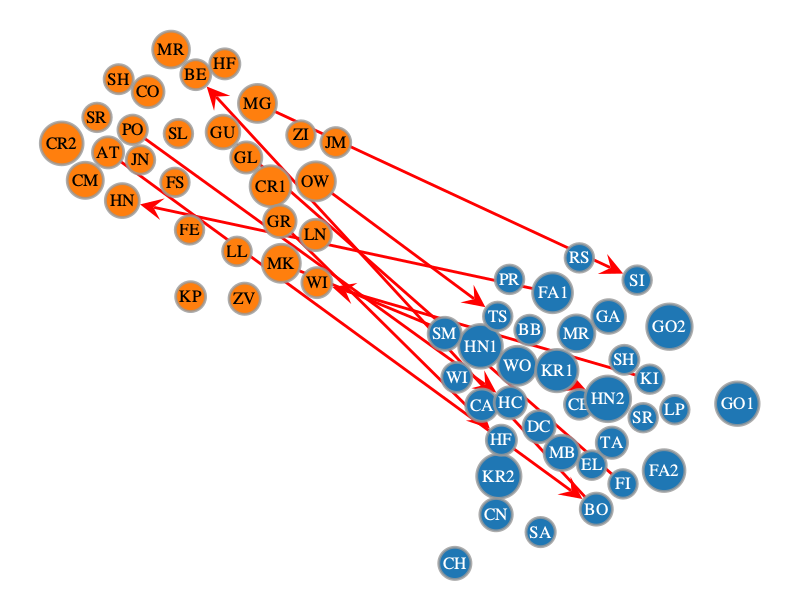
[18]:
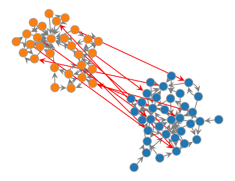
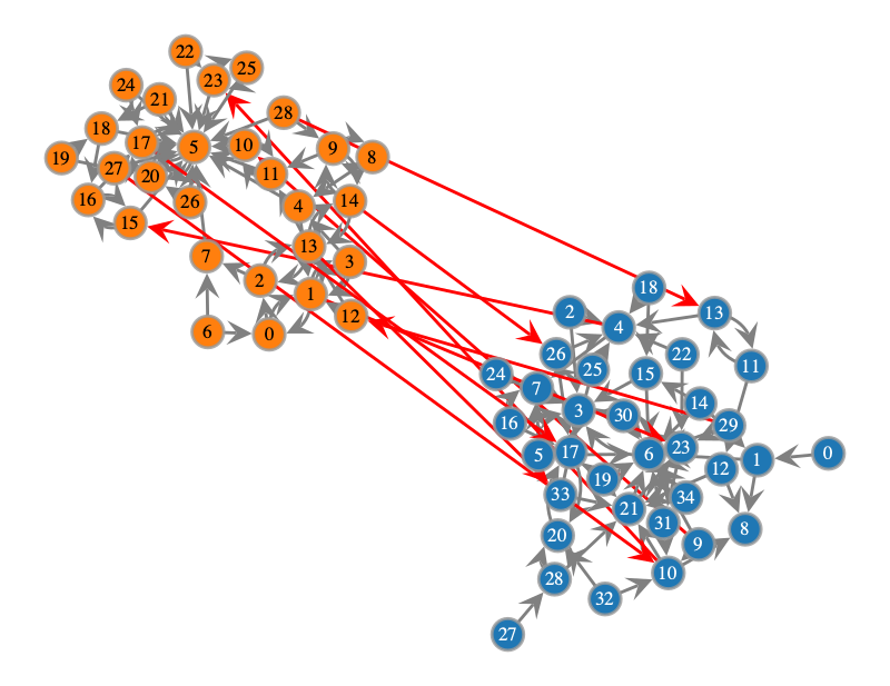
v_cols = onionnet.visualisation.color_nodes(g=onion2.core.graph, prop_name='layer', generate_legend=True)
e_cols = onionnet.visualisation.color_edges(g=onion2.core.graph, prop_name='interlayer', method='boolean', generate_legend=True)

print(v_cols)
print(e_cols)

graph_draw(onion2.core.graph,
           pos=pos_sfdp,
           output_size=(400, 400),
           vertex_fill_color=v_cols['v_color'],
           edge_color=e_cols['e_color'])
{'v_color': <VertexPropertyMap object with value type 'vector<double>', for Graph 0x161d8ac30, at 0x161dc1f40>, 'legend_node_color': {0: (np.float64(0.12156862745098039), np.float64(0.4666666666666667), np.float64(0.7058823529411765), 1.0), 1: (np.float64(1.0), np.float64(0.4980392156862745), np.float64(0.054901960784313725), 1.0)}}
{'e_color': <EdgePropertyMap object with value type 'vector<double>', for Graph 0x161d8ac30, at 0x161ca1730>, 'legend_edge_color': {'True': (1.0, 0.0, 0.0, 1.0), 'False': (0.5, 0.5, 0.5, 1.0)}}
[18]:
<VertexPropertyMap object with value type 'vector<double>', for Graph 0x161d8ac30, at 0x161d0a690>
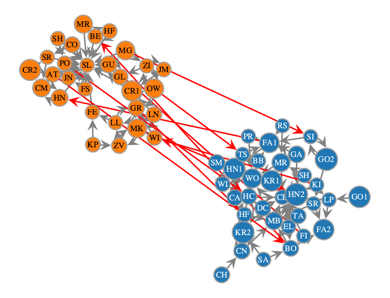
Now it would be good to add labels to this to see the student names. We can do this using vertex_text.
[19]:
graph_draw(onion2.core.graph,
           pos=pos_sfdp,
           output_size=(400, 400),
           vertex_fill_color=v_cols['v_color'],
           edge_color=e_cols['e_color'],
           vertex_text=onion2.core.graph.vp['name'])

[19]:
<VertexPropertyMap object with value type 'vector<double>', for Graph 0x161d8ac30, at 0x161dc05c0>
Oh no! Now all we have is numbers for the students. What has happened here? Let’s look at our original nodes_df
[20]:
df_nodes.groupby(['node_id', 'name']).last().drop(columns='_pos')
[20]:
| layer | ||
|---|---|---|
| node_id | name | |
| 0 | GO1 | grade_1 |
| ZV | grade_2 | |
| 1 | LP | grade_1 |
| MK | grade_2 | |
| 2 | LL | grade_2 |
| ... | ... | ... |
| 30 | KR1 | grade_1 |
| 31 | EL | grade_1 |
| 32 | SA | grade_1 |
| 33 | HF | grade_1 |
| 34 | TA | grade_1 |
64 rows × 1 columns
If we look closely we can also see that these are not the original node_ids in our plot, because in our nodes_id we had some node_ids that were actually the same for student’s with different names!
So why did OnionNet treat these differently and what are the labels on the network plot?
The answer is that behind the scenes OnionNet creates unique nodes based on both the node_id and the layer. Then to improve efficiency, OnionNet encodes these values using the pandas df dtypes by default. So the node numbers we saw before are actually the mappings of these values to a dictionary we have in OnionNet. We can inspect these below.
[21]:
onion2.core.vertex_categorical_mappings.keys()
[21]:
dict_keys(['node_id', 'name', '_pos', 'layer'])
[22]:
onion2.core.vertex_categorical_mappings['layer'].keys()
[22]:
dict_keys(['str_to_int', 'int_to_str'])
[23]:
onion2.core.vertex_categorical_mappings['layer']['str_to_int']
[23]:
{'grade_1': 0, 'grade_2': 1}
[24]:
print(onion2.core.vertex_categorical_mappings.keys())
print(onion2.core.edge_categorical_mappings.keys())
dict_keys(['node_id', 'name', '_pos', 'layer'])
dict_keys(['source_id', 'target_id', 'source_layer', 'target_layer', 'interlayer'])
To convert these integers back into their real values we have to decode them using the decode_property_labels function.
[25]:
extra_vars = ['layer', 'node_id', 'name']
for var in extra_vars:
    onion2.prop_manager.decode_property_labels(
        encoded_prop_type='v',
        encoded_prop_name=var
    )
V property 'layer_decoded' created successfully.
V property 'node_id_decoded' created successfully.
V property 'name_decoded' created successfully.
Note that these properties will be added to the vertex or edge properties of the graph directly
[26]:
print(list(list(onion2.core.graph.vp)))
print(list(list(onion2.core.graph.ep)))
['layer_hash', 'node_id_hash', 'node_id', 'name', '_pos', 'layer', 'layer_decoded', 'node_id_decoded', 'name_decoded']
['source_id', 'target_id', 'source_layer', 'target_layer', 'interlayer']
You won’t see them and they won’t be added to the vertex or edge categorical mappings (because the categorical mappings are just mappings between the encoded values, not the values of the nodes or edge properties directly)
[27]:
print(onion2.core.vertex_categorical_mappings.keys())
print(onion2.core.edge_categorical_mappings.keys())
dict_keys(['node_id', 'name', '_pos', 'layer'])
dict_keys(['source_id', 'target_id', 'source_layer', 'target_layer', 'interlayer'])
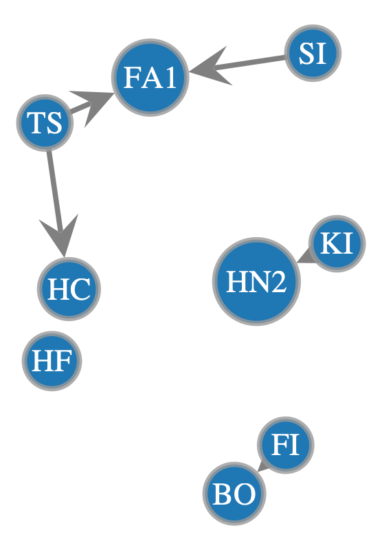
Now that we have the decoded properties in our vertex properties of the graph, we can try drawing the graph again, this time using the name_decoded vertex property
[28]:
graph_draw(onion2.core.graph,
           pos=pos_sfdp,
           output_size=(400, 400),
           vertex_fill_color=v_cols['v_color'],
           edge_color=e_cols['e_color'],
           vertex_text=onion2.core.graph.vp['name_decoded'])

[28]:
<VertexPropertyMap object with value type 'vector<double>', for Graph 0x161d8ac30, at 0x161dc3fb0>
We should also generate a legend for this too, so we know which category is which
[29]:
onionnet.visualisation.get_legend(onion2.core.graph, prop='layer_decoded', title='Layer')
onionnet.visualisation.get_legend(source=e_cols['legend_edge_color'], title='Interlayer')
Filtering the multi-layer network by layers#
Now what if we want to filter the network in some ways, for example get a single layer, or multiple layers?
To filter and view certain layers of the network we can use the OnionNet searcher.view_layers function.
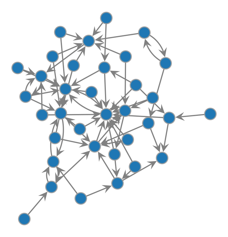
[30]:
filtered_layers_gv = onion2.searcher.view_layers(layer_names=['grade_1'])
filtered_layers_gv
[30]:
<GraphView object, directed, with 35 vertices and 67 edges, 9 internal vertex properties, 5 internal edge properties, edges filtered by (<EdgePropertyMap object with value type 'bool', for Graph 0x161d63e60, at 0x162b66db0>, False), vertices filtered by (<VertexPropertyMap object with value type 'bool', for Graph 0x161d63e60, at 0x162b64350>, False), at 0x161d63e60>
This returns a GraphView object.
We could also just create a vertex property map (but for now we will not use it)
[31]:
filtered_layers_vpm = onion2.searcher.view_layers(layer_names=['grade_1'], return_filter=True)
filtered_layers_vpm
[31]:
<VertexPropertyMap object with value type 'bool', for Graph 0x161d8ac30, at 0x162b52b70>
[32]:
graph_draw(filtered_layers_gv,
           pos=pos_sfdp,
           output_size=(400, 400),
           vertex_fill_color=v_cols['v_color'],
           edge_color=e_cols['e_color']) #,
           #vertex_text=filtered_layers.core.graph.vp['name_decoded'])
[32]:
<VertexPropertyMap object with value type 'vector<double>', for Graph 0x161d63e60, at 0x162b68140>
The graph view has all the same properties as before
[33]:
list(filtered_layers_gv.vertex_properties)
[33]:
['layer_hash',
 'node_id_hash',
 'node_id',
 'name',
 '_pos',
 'layer',
 'layer_decoded',
 'node_id_decoded',
 'name_decoded']
But if you try running the function below you will get an error:
ValueError: could not broadcast input array from shape (64,) into shape (35,)
[34]:
# graph_draw(filtered_layers_gv,
#            pos=pos_sfdp,
#            output_size=(400, 400),
#            vertex_fill_color=v_cols['v_color'],
#            edge_color=e_cols['e_color'],
#            vertex_text=filtered_layers_gv.vp['name_decoded'])
This is because the property maps that we had before for colour of the edges and nodes were for the full graph. Since these were not attached as a vertex or edge property to the graph, the filtered graph layer operation that we did has resulted in the filter being different in shape to the colour property maps.
To overcome this, we have two options:
recompute the vertex or edge properties using the filtered graph
assign the color property maps to the original graph before filtering
Your choice of these depends on whether you think you will be using the property for long or just want it on the fly
Option 1) recalculating property maps#
[35]:
v_cols2 = onionnet.visualisation.color_nodes(g=filtered_layers_gv, prop_name='layer')
e_cols2 = onionnet.visualisation.color_edges(g=filtered_layers_gv, prop_name='interlayer', method='boolean')

print(v_cols2)
print(e_cols2)
{'v_color': <VertexPropertyMap object with value type 'vector<double>', for Graph 0x161d63e60, at 0x162b646b0>, 'legend_node_color': None}
{'e_color': <EdgePropertyMap object with value type 'vector<double>', for Graph 0x161d63e60, at 0x162b6a3c0>, 'legend_edge_color': None}
[36]:
graph_draw(filtered_layers_gv,
           pos=pos_sfdp,
           output_size=(400, 400),
           vertex_fill_color=v_cols2['v_color'],
           edge_color=e_cols2['e_color'],
           vertex_text=filtered_layers_gv.vp['name_decoded'])
[36]:
<VertexPropertyMap object with value type 'vector<double>', for Graph 0x161d63e60, at 0x162b67b00>
Option 2) assigning property maps before filtering#
[37]:
onion2.core.graph.vp['v_color'] = v_cols['v_color']
onion2.core.graph.ep['e_color'] = e_cols['e_color']
[38]:
filtered_layers_gv2 = onion2.searcher.view_layers(layer_names=['grade_1'])
filtered_layers_gv2
[38]:
<GraphView object, directed, with 35 vertices and 67 edges, 10 internal vertex properties, 6 internal edge properties, edges filtered by (<EdgePropertyMap object with value type 'bool', for Graph 0x162bd8350, at 0x162bd8710>, False), vertices filtered by (<VertexPropertyMap object with value type 'bool', for Graph 0x162bd8350, at 0x162bd9730>, False), at 0x162bd8350>
[39]:
print(list(filtered_layers_gv2.vp))
print(list(filtered_layers_gv2.ep))
['layer_hash', 'node_id_hash', 'node_id', 'name', '_pos', 'layer', 'layer_decoded', 'node_id_decoded', 'name_decoded', 'v_color']
['source_id', 'target_id', 'source_layer', 'target_layer', 'interlayer', 'e_color']
[40]:
graph_draw(filtered_layers_gv2,
           pos=pos_sfdp,
           output_size=(400, 400),
           vertex_fill_color=filtered_layers_gv2.vp['v_color'],
           edge_color=filtered_layers_gv2.ep['e_color'],
           vertex_text=filtered_layers_gv2.vp['name_decoded'])

[40]:
<VertexPropertyMap object with value type 'vector<double>', for Graph 0x162bd8350, at 0x162bd9c10>
Searching and filtering the network by nodes#
[41]:
graph_draw(onion2.core.graph,
           pos=pos_sfdp,
           output_size=(400, 400),
           vertex_fill_color=v_cols['v_color'],
           edge_color=e_cols['e_color'],
           vertex_text=onion2.core.graph.vp['node_id'])

graph_draw(onion2.core.graph,
           pos=pos_sfdp,
           output_size=(400, 400),
           vertex_fill_color=v_cols['v_color'],
           edge_color=e_cols['e_color'],
           vertex_text=onion2.core.graph.vp['name_decoded'])

[41]:
<VertexPropertyMap object with value type 'vector<double>', for Graph 0x161d8ac30, at 0x162b65c40>
Now we can run a search
[42]:
node_search_res = onion2.searcher.search(show_plot=False)

graph_draw(node_search_res,
           pos=pos_sfdp,
           output_size=(400, 400),
           vertex_fill_color=node_search_res.vp['v_color'],
           edge_color=node_search_res.ep['e_color'],
           vertex_text=node_search_res.vp['name_decoded'])
Filtered graph contains 11 vertices and 18 edges.
[42]:
<VertexPropertyMap object with value type 'vector<double>', for Graph 0x1619b3530, at 0x162b51a90>
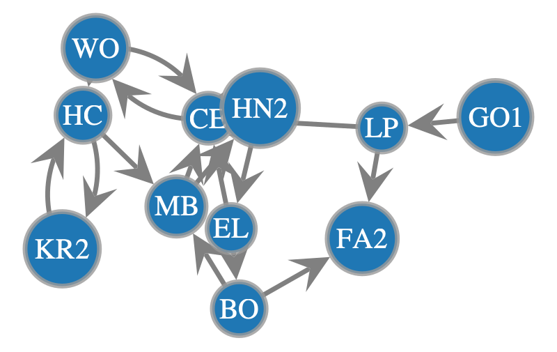
By default, you will see that search used the 0 index starting node if we don’t provide it with any more information. Furthermore, by default it only traverses downstream of the network up to 5 steps. We could try extending this.
[43]:
node_search_res = onion2.searcher.search(show_plot=False,
                                         max_dist=7)

graph_draw(node_search_res,
           pos=pos_sfdp,
           output_size=(400, 400),
           vertex_fill_color=node_search_res.vp['v_color'],
           edge_color=node_search_res.ep['e_color'],
           vertex_text=node_search_res.vp['name_decoded'])
Filtered graph contains 15 vertices and 26 edges.
[43]:
<VertexPropertyMap object with value type 'vector<double>', for Graph 0x162b67140, at 0x161d636e0>
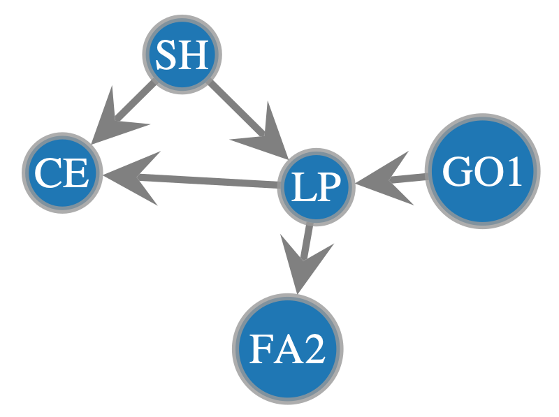
What if we extend a bit more?
[44]:
node_search_res = onion2.searcher.search(show_plot=False,
                                         max_dist=10)

graph_draw(node_search_res,
           pos=pos_sfdp,
           output_size=(400, 400),
           vertex_fill_color=node_search_res.vp['v_color'],
           edge_color=node_search_res.ep['e_color'],
           vertex_text=node_search_res.vp['name_decoded'])
Filtered graph contains 17 vertices and 33 edges.
[44]:
<VertexPropertyMap object with value type 'vector<double>', for Graph 0x162b51580, at 0x162b51160>
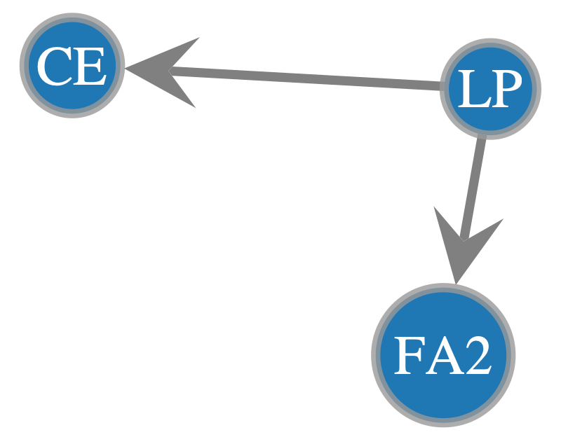
We could also try starting with a different index
[45]:
node_search_res = onion2.searcher.search(show_plot=False,
                                         start_node_idx=1,
                                         max_dist=1)

graph_draw(node_search_res,
           pos=pos_sfdp,
           output_size=(400, 400),
           vertex_fill_color=node_search_res.vp['v_color'],
           edge_color=node_search_res.ep['e_color'],
           vertex_text=node_search_res.vp['name_decoded'])
Filtered graph contains 3 vertices and 2 edges.
[45]:
<VertexPropertyMap object with value type 'vector<double>', for Graph 0x162bda8a0, at 0x162b51580>
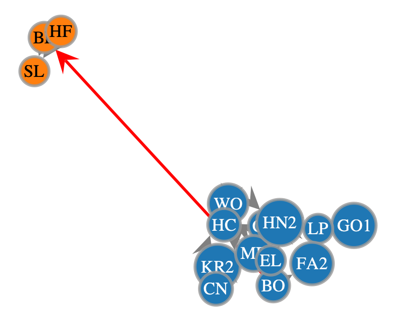
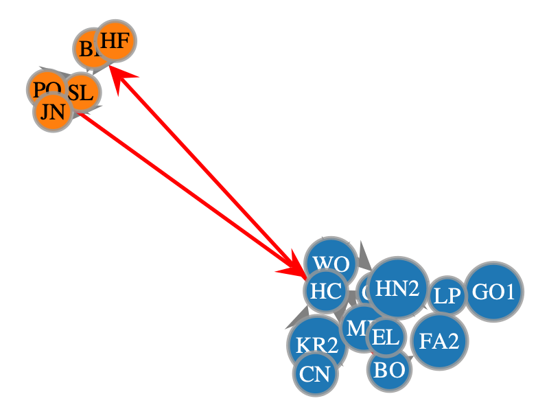
And we could also search upstream or bidirectionally
[46]:
node_search_res = onion2.searcher.search(show_plot=False,
                                         start_node_idx=1,
                                         direction='bi',
                                         max_dist=1)

graph_draw(node_search_res,
           pos=pos_sfdp,
           output_size=(400, 400),
           vertex_fill_color=node_search_res.vp['v_color'],
           edge_color=node_search_res.ep['e_color'],
           vertex_text=node_search_res.vp['name_decoded'])
Filtered graph contains 5 vertices and 5 edges.
[46]:
<VertexPropertyMap object with value type 'vector<double>', for Graph 0x162bda6f0, at 0x162b67020>
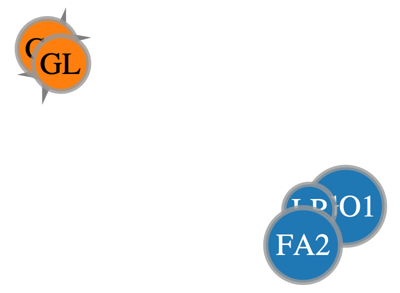
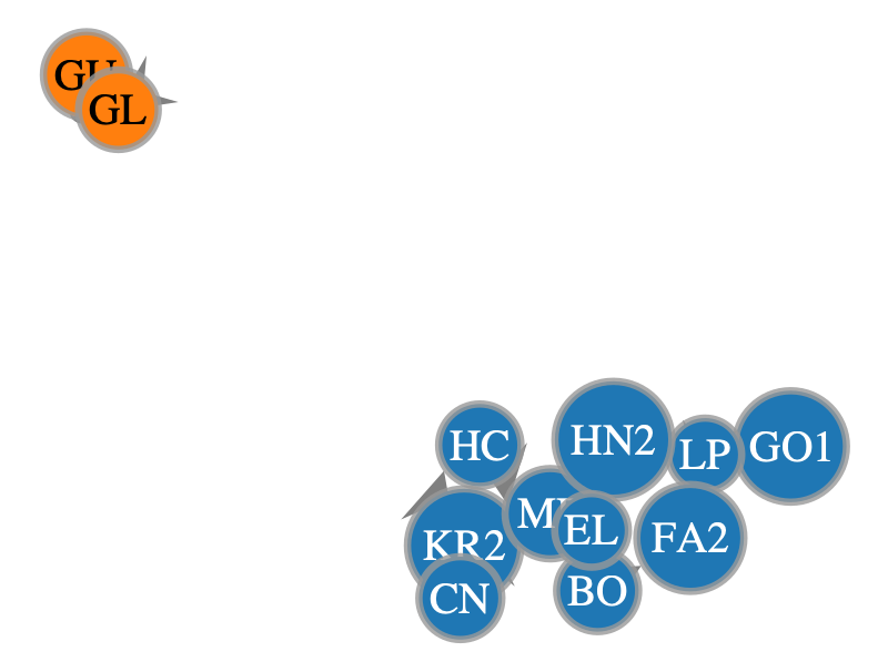
We could also get all nodes that meet a certain condition, such as all nodes that are in a list of names.
[47]:
random_friends_gv = onion2.searcher.filter_view_by_property(
    prop_name='name_decoded',
    target_value=['GO1', 'LP', 'FA2','GL','GU'])

graph_draw(random_friends_gv,
           pos=pos_sfdp,
           output_size=(400, 400),
           vertex_fill_color=random_friends_gv.vp['v_color'],
           edge_color=random_friends_gv.ep['e_color'],
           vertex_text=random_friends_gv.vp['name_decoded'])
[47]:
<VertexPropertyMap object with value type 'vector<double>', for Graph 0x162b51e50, at 0x161dc0a70>
[48]:
list(random_friends_gv.vertices())
[48]:
[<Vertex object with index '0' at 0x162b5ad40>,
 <Vertex object with index '1' at 0x162b5a8c0>,
 <Vertex object with index '8' at 0x162b5b3c0>,
 <Vertex object with index '45' at 0x162b5bac0>,
 <Vertex object with index '46' at 0x162b5a9c0>]
[49]:
list(random_friends_gv.vertices())[0].out_degree()
[49]:
1
We could also filter the graph according to some edge attribute condition. In this case we will test with interlayer, to only show the connections between kids in the 1st and 2nd grade.
[50]:
interlayer_friends_gv = onion2.searcher.filter_view_by_property(
    prop_name='interlayer',
    target_value=True,
    dim='e')

graph_draw(interlayer_friends_gv,
           pos=pos_sfdp,
           output_size=(400, 400),
           vertex_fill_color=interlayer_friends_gv.vp['v_color'],
           edge_color=interlayer_friends_gv.ep['e_color'],
           vertex_text=interlayer_friends_gv.vp['name_decoded'])
[50]:
<VertexPropertyMap object with value type 'vector<double>', for Graph 0x162bda1e0, at 0x161d8b7d0>
Note that by default this function doesn’t automatically remove the nodes that are isolated with no edges connecting them. If we want to do that we should specify prune_isolated=True
[51]:
interlayer_friends_gv_pruned = onion2.searcher.filter_view_by_property(
    prop_name='interlayer',
    target_value=True,
    dim='e',
    prune_isolated=True)

graph_draw(interlayer_friends_gv_pruned,
           pos=pos_sfdp,
           output_size=(400, 400),
           vertex_fill_color=interlayer_friends_gv_pruned.vp['v_color'],
           edge_color=interlayer_friends_gv_pruned.ep['e_color'],
           vertex_text=interlayer_friends_gv_pruned.vp['name_decoded'])
[51]:
<VertexPropertyMap object with value type 'vector<double>', for Graph 0x162c10bf0, at 0x161dc1880>
Another way that we can filter the graph, if we wish to use more advanced logic, is to use lambda functions. OnionNet provides a helper function as well to combine these functions. For instance, we could filter to have either grade_1 or grade_2:
[52]:
filter1 = lambda v: onion2.core.graph.vp['layer_decoded'][v] == 'grade_1'
filter2 = lambda v: onion2.core.graph.vp['layer_decoded'][v] == 'grade_2'
filtered_view = onion2.searcher.compose_filters([filter1, filter2], mode="or")

graph_draw(filtered_view,
           pos=pos_sfdp,
           output_size=(400, 400),
           vertex_fill_color=filtered_view.vp['v_color'],
           edge_color=filtered_view.ep['e_color'],
           vertex_text=filtered_view.vp['name_decoded'])
[52]:
<VertexPropertyMap object with value type 'vector<double>', for Graph 0x162c10d10, at 0x162bd9af0>
Or filter to the interlayer friends from before, but this time only show the ones in grade_1, we could try the method below…
[53]:
filter1 = lambda v: onion2.core.graph.vp['layer_decoded'][v] == 'grade_1'
filter2 = lambda v: onion2.core.graph.vp['name_decoded'][v] in {interlayer_friends_gv_pruned.vp['name_decoded'][item] for item in interlayer_friends_gv_pruned.vertices()}
filtered_view = onion2.searcher.compose_filters([filter1, filter2], mode="and")

graph_draw(filtered_view,
           pos=pos_sfdp,
           output_size=(400, 400),
           vertex_fill_color=filtered_view.vp['v_color'],
           edge_color=filtered_view.ep['e_color'],
           vertex_text=filtered_view.vp['name_decoded'])
[53]:
<VertexPropertyMap object with value type 'vector<double>', for Graph 0x162c10680, at 0x162b53c20>
But if we inspect this carefully, we will see that the blue grade 1 node labelled WI has been included, even though it wasn’t in interlayer_friends_gv_pruned! Why is this?
The answer is that because the method above used the decoded_names, there was another child called WI in the other grade that was also included in the interlayer_friends_gv_pruned. So the AND condition we used for the filtered condition included both WI children, but only selected the one in Grade 1. Also if we used something like the node_id this problem would have been even more widespread, because many of the nodes share the same ID’s but are in different layers!
This is a cautionary tale: we need to be careful about what conditions we are using for filtering and think about possible edge cases. Luckily in this case we were able to diagnose the problem, but on a much larger or complex graph you can imagine this could be much more difficult.
To fix this we will use the actual vertices themselves, which are handled more unambiguously by graph-tool.
[54]:
filter1 = lambda v: onion2.core.graph.vp['layer_decoded'][v] == 'grade_1'
pruned_vs = set(interlayer_friends_gv_pruned.vertices())
filter2 = lambda v: v in pruned_vs

filtered_view = onion2.searcher.compose_filters([filter1, filter2], mode="and")

graph_draw(filtered_view,
           pos=pos_sfdp,
           output_size=(400, 400),
           vertex_fill_color=filtered_view.vp['v_color'],
           edge_color=filtered_view.ep['e_color'],
           vertex_text=filtered_view.vp['name_decoded'])
[54]:
<VertexPropertyMap object with value type 'vector<double>', for Graph 0x162c10b60, at 0x162b68050>
[55]:
filtered_view
[55]:
<GraphView object, directed, with 9 vertices and 5 edges, 10 internal vertex properties, 6 internal edge properties, edges filtered by (<EdgePropertyMap object with value type 'bool', for Graph 0x162c10b60, at 0x162c11190>, False), vertices filtered by (<VertexPropertyMap object with value type 'bool', for Graph 0x162c10b60, at 0x162c108c0>, False), at 0x162c10b60>
Great, now we have the same nodes from earlier that were in the interlayer_friends_gv_pruned view, but this time only for those in Grade 1.
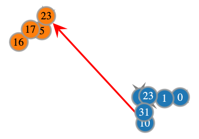
Shortest paths#
If we want to find the shortest path between a given node and a collection of other nodes we can do it using the compute_on_shortest() method.
[56]:
# Compute shortest path between the source idx and the target indices - returns a vertex property map
shortest_path_vpm = onion2.searcher.compute_on_shortest(source=0, targets=[51,52], return_gv=False)
# Filter a graphview to the
shortest_path_gv = gt.GraphView(onion2.core.graph, vfilt=shortest_path_vpm)

# Show the same shortest path graphview with different attributes as the nodes
# Node ID
graph_draw(shortest_path_gv,
           pos=pos_sfdp,
           output_size=(200, 200),
           vertex_fill_color=shortest_path_gv.vp['v_color'],
           edge_color=shortest_path_gv.ep['e_color'],
           vertex_text=shortest_path_gv.vp['node_id'])
# Vertex Index
graph_draw(shortest_path_gv,
           pos=pos_sfdp,
           output_size=(200, 200),
           vertex_fill_color=shortest_path_gv.vp['v_color'],
           edge_color=shortest_path_gv.ep['e_color'],
           vertex_text=onion2.core.graph.vertex_index)
# Name (decoded)
graph_draw(shortest_path_gv,
           pos=pos_sfdp,
           output_size=(200, 200),
           vertex_fill_color=shortest_path_gv.vp['v_color'],
           edge_color=shortest_path_gv.ep['e_color'],
           vertex_text=shortest_path_gv.vp['name_decoded'])
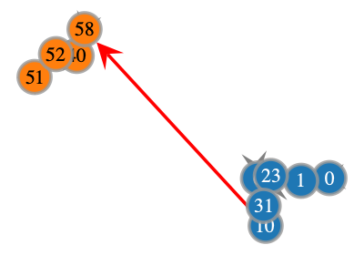
[56]:
<VertexPropertyMap object with value type 'vector<double>', for Graph 0x161dc26c0, at 0x161d63050>
Notice above how the vertex index is different to the category mapping of the node, which we should keep in mind.
[57]:
print(onion2.get_vertex_by_name_tuple(layer_name='grade_1', node_id_str='0'))
print(onion2.get_vertex_by_name_tuple(layer_name='grade_2', node_id_str='0'))
0
35
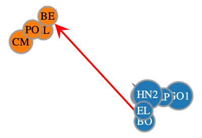
Ok now what if we want to find the path between a particular index and a bunch of different indices? We can use our list(random_friends_gv.vertices()) from earlier to find connections here between these
[58]:
random_friends_gv_idxlist = [int(item) for item in random_friends_gv.vertices()]

shortest_path_vpm2 = onion2.searcher.compute_on_shortest(source=20, targets=random_friends_gv_idxlist, return_gv=False)

shortest_path_gv2 = gt.GraphView(onion2.core.graph, vfilt=shortest_path_vpm2)


graph_draw(shortest_path_gv2,
           pos=pos_sfdp,
           output_size=(400, 400),
           vertex_fill_color=shortest_path_gv2.vp['v_color'],
           edge_color=shortest_path_gv2.ep['e_color'],
           vertex_text=shortest_path_gv2.vp['name_decoded'])
[58]:
<VertexPropertyMap object with value type 'vector<double>', for Graph 0x162bda240, at 0x162b52d80>
[59]:
onion2.core.graph.vp['node_id'].a
[59]:
PropertyArray([ 0,  1,  2,  3,  4,  5,  6,  7,  8,  9, 10, 11, 12, 13, 14,
               15, 16, 17, 18, 19, 20, 21, 22, 23, 24, 25, 26, 27, 28, 29,
               30, 31, 32, 33, 34,  0,  1,  2,  3,  4,  5,  6,  7,  8,  9,
               10, 11, 12, 13, 14, 15, 16, 17, 18, 19, 20, 21, 22, 23, 24,
               25, 26, 27, 28], dtype=int32)
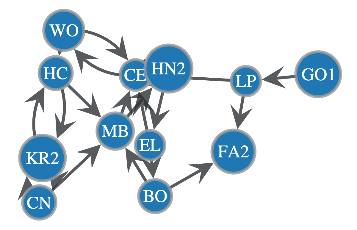
What about combining operations? So filtering to a certain layer of the network and then performing a search.
[60]:
onion2.view_layers(['grade_1'])
[60]:
<GraphView object, directed, with 35 vertices and 67 edges, 10 internal vertex properties, 6 internal edge properties, edges filtered by (<EdgePropertyMap object with value type 'bool', for Graph 0x162bda3f0, at 0x162c2c200>, False), vertices filtered by (<VertexPropertyMap object with value type 'bool', for Graph 0x162bda3f0, at 0x162c2c590>, False), at 0x162bda3f0>
[61]:
filter_lay = onion2.view_layers(['grade_1'])
search_res = onion2.searcher.search(g=filter_lay,
                                    direction='bi',
                                    max_dist=20,
                                    show_plot=False
                                    )
v_colors = onionnet.visualisation.color_nodes(g=search_res, prop_name='layer')['v_color']
search_res.vp['v_color'] = v_colors
graph_draw(
    search_res,
    vertex_text=search_res.vp['name_decoded'],
    pos=pos_sfdp,
    vertex_fill_color=search_res.vp['v_color']
    )
Filtered graph contains 12 vertices and 21 edges.
[61]:
<VertexPropertyMap object with value type 'vector<double>', for Graph 0x161dc21b0, at 0x162b93aa0>
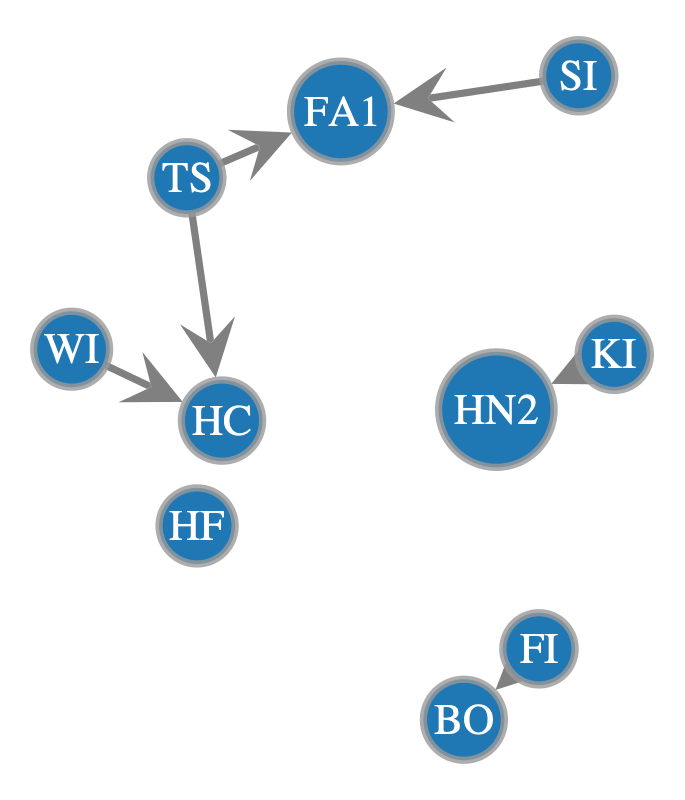
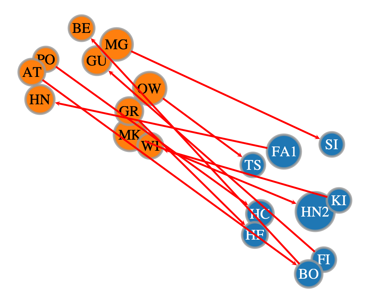
Bipartite graph creation#
Earlier on we experimented with filtering the interlayers using lambda and some other functions. In OnionNet there is actually a dedicated way to do this kind of analysis between two layers of the network. This ignores intra-layer connections and filters to only nodes involved in the inter-layer links between these two layers, effectively creating a bipartite network. To do this use the filter_edges_between_categories function.
[62]:
layer_1 = 'grade_1'
layer_2 = 'grade_2'
bipartite_gv = onion2.filter_edges_between_categories(source_label=layer_1, target_label=layer_2, mode='both')
bipartite_gv
[62]:
<GraphView object, directed, with 19 vertices and 10 edges, 10 internal vertex properties, 6 internal edge properties, edges filtered by (<EdgePropertyMap object with value type 'bool', for Graph 0x162b93140, at 0x162b92270>, False), vertices filtered by (<VertexPropertyMap object with value type 'bool', for Graph 0x162b93140, at 0x162b922a0>, False), at 0x162b93140>
[63]:
graph_draw(bipartite_gv,
           edge_pen_width=3.0,
           pos=pos_sfdp,
           vertex_text=search_res.vp['name_decoded'],
           vertex_fill_color=bipartite_gv.vp['v_color'],
           edge_color=e_cols['e_color'],
           nodesfirst=True)
[63]:
<VertexPropertyMap object with value type 'vector<double>', for Graph 0x162b93140, at 0x162c12690>
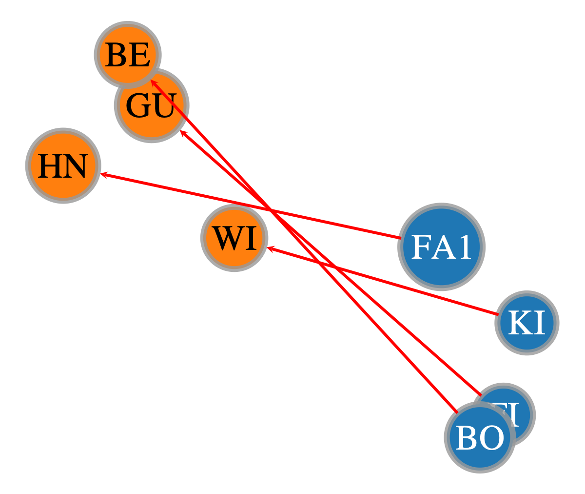
What if we wanted to filter and show connections only between grade_1 and grade_2 but in a unidirectional manner?
We can use the same filter_edges_between_categories method but with the forward method (note the reverse method is also supported).
[64]:
bipartite_gv_1way = onion2.filter_edges_between_categories(source_label=layer_1, target_label=layer_2, mode='forward')
bipartite_gv_1way
[64]:
<GraphView object, directed, with 8 vertices and 4 edges, 10 internal vertex properties, 6 internal edge properties, edges filtered by (<EdgePropertyMap object with value type 'bool', for Graph 0x162b53b30, at 0x162b53170>, False), vertices filtered by (<VertexPropertyMap object with value type 'bool', for Graph 0x162b53b30, at 0x162b52210>, False), at 0x162b53b30>
[65]:
graph_draw(bipartite_gv_1way,
           edge_pen_width=3.0,
           pos=pos_sfdp,
           vertex_text=search_res.vp['name_decoded'],
           vertex_fill_color=bipartite_gv_1way.vp['v_color'],
           edge_color=e_cols['e_color'],
           nodesfirst=True)
[65]:
<VertexPropertyMap object with value type 'vector<double>', for Graph 0x162b53b30, at 0x162c12c90>
[66]:
onionnet.exporter.export_info(bipartite_gv_1way)
[66]:
| v_int | layer_hash | node_id_hash | node_id | name | _pos | layer | layer_decoded | node_id_decoded | name_decoded | v_color | |
|---|---|---|---|---|---|---|---|---|---|---|---|
| 0 | 4 | 0 | 4 | 4 | 4 | 4 | 0 | grade_1 | 4 | FA1 | [0.12156862745098039, 0.4666666666666667, 0.70... |
| 1 | 9 | 0 | 8 | 9 | 9 | 9 | 0 | grade_1 | 9 | FI | [0.12156862745098039, 0.4666666666666667, 0.70... |
| 2 | 10 | 0 | 9 | 10 | 10 | 10 | 0 | grade_1 | 10 | BO | [0.12156862745098039, 0.4666666666666667, 0.70... |
| 3 | 29 | 0 | 28 | 29 | 29 | 29 | 0 | grade_1 | 29 | KI | [0.12156862745098039, 0.4666666666666667, 0.70... |
| 4 | 45 | 1 | 9 | 10 | 45 | 45 | 1 | grade_2 | 10 | GU | [1.0, 0.4980392156862745, 0.054901960784313725... |
| 5 | 47 | 1 | 11 | 12 | 16 | 47 | 1 | grade_2 | 12 | WI | [1.0, 0.4980392156862745, 0.054901960784313725... |
| 6 | 50 | 1 | 14 | 15 | 49 | 50 | 1 | grade_2 | 15 | HN | [1.0, 0.4980392156862745, 0.054901960784313725... |
| 7 | 58 | 1 | 22 | 23 | 55 | 58 | 1 | grade_2 | 23 | BE | [1.0, 0.4980392156862745, 0.054901960784313725... |
[67]:
onionnet.exporter.export_info(bipartite_gv_1way, mode='e')
[67]:
| e_id | source | target | source_id | target_id | source_layer | target_layer | interlayer | e_color | |
|---|---|---|---|---|---|---|---|---|---|
| 0 | 132 | 4 | 50 | 4 | 14 | 0 | 1 | 1 | [1.0, 0.0, 0.0, 1.0] |
| 1 | 133 | 9 | 45 | 8 | 9 | 0 | 1 | 1 | [1.0, 0.0, 0.0, 1.0] |
| 2 | 135 | 10 | 58 | 9 | 7 | 0 | 1 | 1 | [1.0, 0.0, 0.0, 1.0] |
| 3 | 129 | 29 | 47 | 28 | 11 | 0 | 1 | 1 | [1.0, 0.0, 0.0, 1.0] |
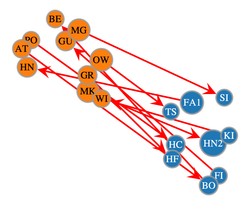
Going back to the fully bipartite (both way graph) could also view these with a more spread out layout
[68]:
graph_draw(bipartite_gv,
           edge_pen_width=3.0,
           vertex_text=search_res.vp['name_decoded'],
           vertex_fill_color=bipartite_gv.vp['v_color'],
           edge_color=e_cols['e_color'],
           nodesfirst=True)

[68]:
<VertexPropertyMap object with value type 'vector<double>', for Graph 0x162b93140, at 0x162c12420>
Or we can even create a special bipartite layout to do this
[69]:
pos_bipartite = onionnet.visualisation.layout_by_layer(bipartite_gv)

graph_draw(bipartite_gv,
           edge_pen_width=3.0,
           pos=pos_bipartite,
           vertex_text=search_res.vp['name_decoded'],
           vertex_fill_color=bipartite_gv.vp['v_color'],
           edge_color=e_cols['e_color'],
           nodesfirst=True)
[69]:
<VertexPropertyMap object with value type 'vector<double>', for Graph 0x162b93140, at 0x162c132c0>
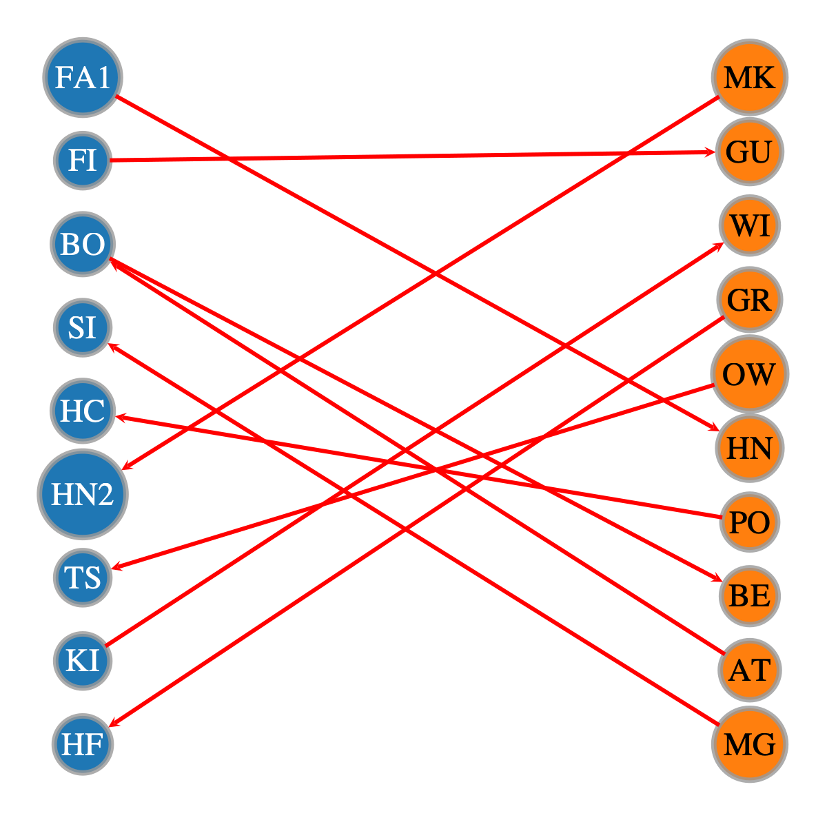
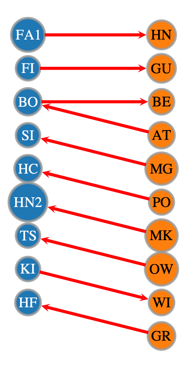
We can also order this to improve the ability to discern patterns in the connections. This allows us to more easily see the double connection between BO.
[70]:
pos_bipartite_ordered = onionnet.visualisation.bipartite_ordered_layout(bipartite_gv, left_val='grade_1', right_val='grade_2',
                                                                        vertical_spacing=100, horizontal_spacing=400)

graph_draw(bipartite_gv,
           edge_pen_width=5.0,
           pos=pos_bipartite_ordered,
           vertex_text=search_res.vp['name_decoded'],
           vertex_fill_color=bipartite_gv.vp['v_color'],
           edge_color=e_cols['e_color'],
           nodesfirst=True)
[70]:
<VertexPropertyMap object with value type 'vector<double>', for Graph 0x162b93140, at 0x162b52540>
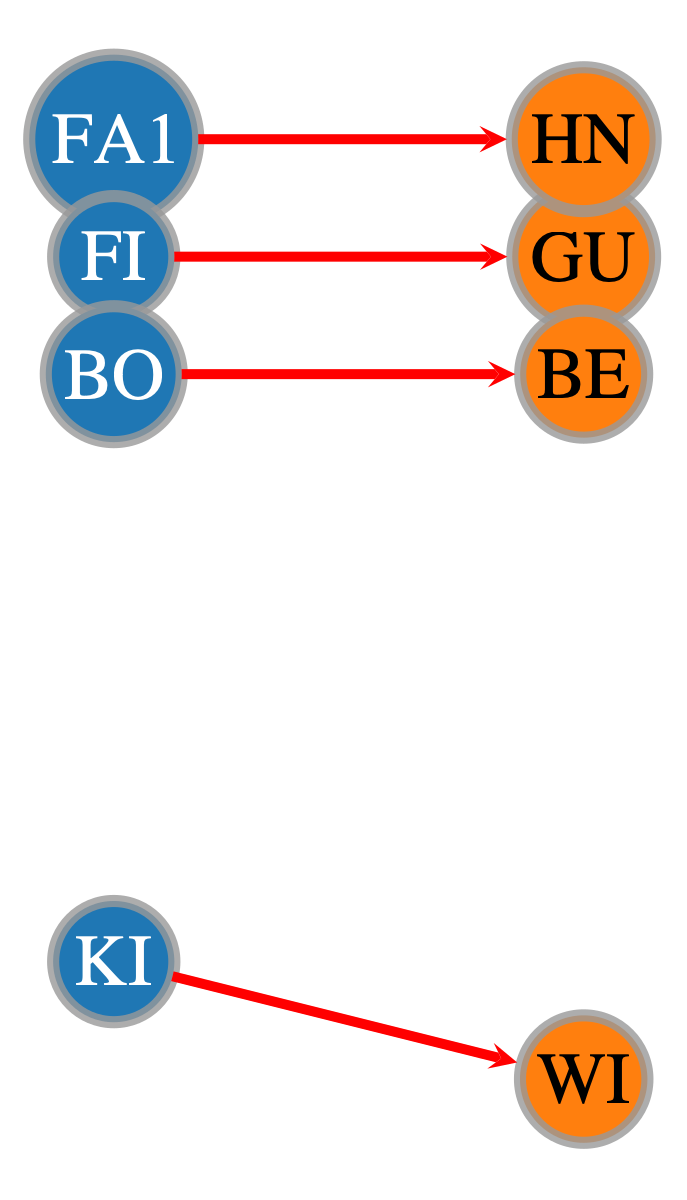
Again, we could also inspect only those that were filtered between one layer and the other
[71]:
graph_draw(bipartite_gv_1way,
           edge_pen_width=5.0,
           pos=pos_bipartite_ordered,
           vertex_text=search_res.vp['name_decoded'],
           vertex_fill_color=bipartite_gv_1way.vp['v_color'],
           edge_color=e_cols['e_color'],
           nodesfirst=True)
[71]:
<VertexPropertyMap object with value type 'vector<double>', for Graph 0x162b53b30, at 0x162b91a00>
Viewing the OnionNet MetaGraph#
This simple example should have been relatively easy to follow: we only had two layers and some connections within and between them. Even still it could be useful visualising this in an overview.
Furthermore, if we start working with say 5, 10, or even more than 20 layers, with complex relationships between them, visualising and interpreting this will be crucial.
That’s where the onionnet.analytics module comes in, and specifically layer_stats and plot_layer_metagraph.
[73]:
nodes_by_layer, edges_by_pair = layer_stats(
    df_nodes=df_nodes,
    df_edges=df_edges_with_friends,
    print_tables=True
)
Node counts by layer:
| count | |
|---|---|
| layer | |
| grade_1 | 35 |
| grade_2 | 29 |
Interlayer edge count: 10
Edge counts by (source_layer, target_layer):
| edges | ||
|---|---|---|
| source_layer | target_layer | |
| grade_1 | grade_1 | 67 |
| grade_2 | grade_2 | 59 |
| grade_1 | 6 | |
| grade_1 | grade_2 | 4 |
[74]:
plot_layer_metagraph(
    edges_by_pair,
    nodes_by_layer=nodes_by_layer,
    node_scaler="log",
    edge_scaler="log",
    edge_width_range=(5, 10),
    show_labels=True,
    node_size_range=(14, 25),
    show_edge_counts=True,
    show_node_counts=True,
    output_size=(1000, 1000),
)
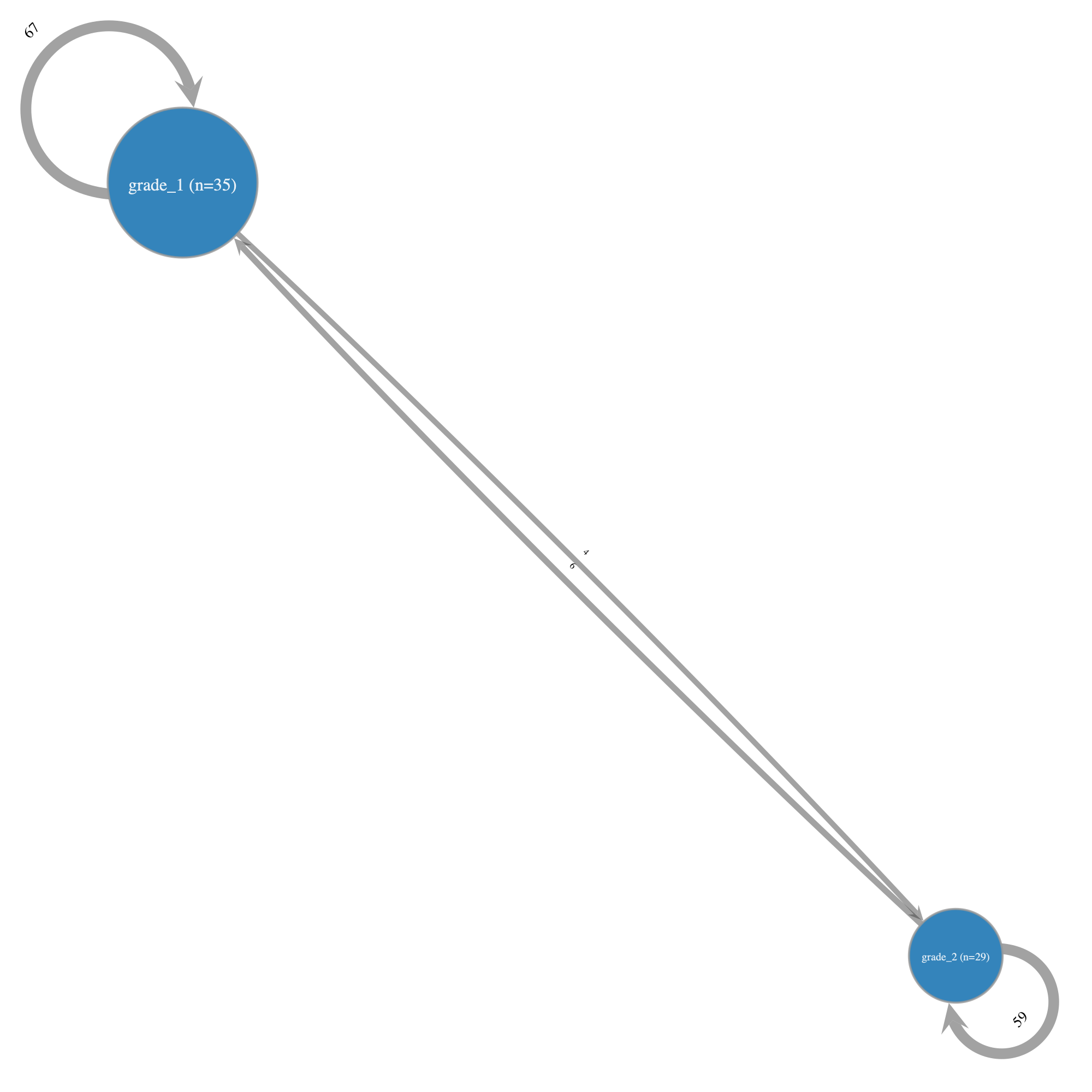
This graph, which by default is relatively proportionate to the underlying node and edge membership, confirms that there were more students in Grade 1 (35) than Grade 2 (29). Furthermore, we’re able to see the exact number of friendships between the two grades in each direction, as well as the number of friendships within the same grades.
Again, in this simple example the utility of such a MetaGraph may not be obvious. However we strongly recommend making use of these MetaGraphs early on in the analysis, such as straight after data loading, since it can greatly help get an understanding of the overall network and any relationships that may be worth considering.
Exporting filtered graphs#
What if we want to now export the data from our filtered network into a dataframe or list, etc.? OnionNet includes a function to do just that: export_info(). By default this will include all node properties. Note however that they will be in the encoded integer format unless we have already decoded certain properties, like we did for name_decoded earlier.
[75]:
onionnet.exporter.export_info(bipartite_gv_1way, mode='v')
[75]:
| v_int | layer_hash | node_id_hash | node_id | name | _pos | layer | layer_decoded | node_id_decoded | name_decoded | v_color | |
|---|---|---|---|---|---|---|---|---|---|---|---|
| 0 | 4 | 0 | 4 | 4 | 4 | 4 | 0 | grade_1 | 4 | FA1 | [0.12156862745098039, 0.4666666666666667, 0.70... |
| 1 | 9 | 0 | 8 | 9 | 9 | 9 | 0 | grade_1 | 9 | FI | [0.12156862745098039, 0.4666666666666667, 0.70... |
| 2 | 10 | 0 | 9 | 10 | 10 | 10 | 0 | grade_1 | 10 | BO | [0.12156862745098039, 0.4666666666666667, 0.70... |
| 3 | 29 | 0 | 28 | 29 | 29 | 29 | 0 | grade_1 | 29 | KI | [0.12156862745098039, 0.4666666666666667, 0.70... |
| 4 | 45 | 1 | 9 | 10 | 45 | 45 | 1 | grade_2 | 10 | GU | [1.0, 0.4980392156862745, 0.054901960784313725... |
| 5 | 47 | 1 | 11 | 12 | 16 | 47 | 1 | grade_2 | 12 | WI | [1.0, 0.4980392156862745, 0.054901960784313725... |
| 6 | 50 | 1 | 14 | 15 | 49 | 50 | 1 | grade_2 | 15 | HN | [1.0, 0.4980392156862745, 0.054901960784313725... |
| 7 | 58 | 1 | 22 | 23 | 55 | 58 | 1 | grade_2 | 23 | BE | [1.0, 0.4980392156862745, 0.054901960784313725... |
We can also do the same for edges
[76]:
onionnet.exporter.export_info(bipartite_gv_1way, mode='e')
[76]:
| e_id | source | target | source_id | target_id | source_layer | target_layer | interlayer | e_color | |
|---|---|---|---|---|---|---|---|---|---|
| 0 | 132 | 4 | 50 | 4 | 14 | 0 | 1 | 1 | [1.0, 0.0, 0.0, 1.0] |
| 1 | 133 | 9 | 45 | 8 | 9 | 0 | 1 | 1 | [1.0, 0.0, 0.0, 1.0] |
| 2 | 135 | 10 | 58 | 9 | 7 | 0 | 1 | 1 | [1.0, 0.0, 0.0, 1.0] |
| 3 | 129 | 29 | 47 | 28 | 11 | 0 | 1 | 1 | [1.0, 0.0, 0.0, 1.0] |
Note the differences between source and targets.
This isn’t super informative to our human eyes so let’s bulk decode all properties then export it.
[77]:
onion2.decode_property_labels_bulk(df=df_nodes, encoded_prop_type='v',)
node_id prop left as is, no decoding needed (not an object type)
V property 'name_decoded' created successfully.
V property '_pos_decoded' created successfully.
V property 'layer_decoded' created successfully.
[78]:
onion2.decode_property_labels_bulk(df=df_edges_with_friends, encoded_prop_type='e')
source_id prop left as is, no decoding needed (not an object type)
target_id prop left as is, no decoding needed (not an object type)
E property 'source_layer_decoded' created successfully.
E property 'target_layer_decoded' created successfully.
interlayer prop left as is, no decoding needed (not an object type)
Now that we’ve decoded the properties we need to rerun the filtering
[79]:
bipartite_gv_1way = onion2.filter_edges_between_categories(source_label=layer_1, target_label=layer_2, mode='forward')
bipartite_gv_1way
[79]:
<GraphView object, directed, with 8 vertices and 4 edges, 11 internal vertex properties, 8 internal edge properties, edges filtered by (<EdgePropertyMap object with value type 'bool', for Graph 0x162bd8170, at 0x162c2e3f0>, False), vertices filtered by (<VertexPropertyMap object with value type 'bool', for Graph 0x162bd8170, at 0x162bd8e00>, False), at 0x162bd8170>
[80]:
onionnet.exporter.export_info(bipartite_gv_1way, mode='v')
[80]:
| v_int | layer_hash | node_id_hash | node_id | name | _pos | layer | layer_decoded | node_id_decoded | name_decoded | v_color | _pos_decoded | |
|---|---|---|---|---|---|---|---|---|---|---|---|---|
| 0 | 4 | 0 | 4 | 4 | 4 | 4 | 0 | grade_1 | 4 | FA1 | [0.12156862745098039, 0.4666666666666667, 0.70... | array([-3.19714822, 2.96207321]) |
| 1 | 9 | 0 | 8 | 9 | 9 | 9 | 0 | grade_1 | 9 | FI | [0.12156862745098039, 0.4666666666666667, 0.70... | array([-2.66954048, 1.51927661]) |
| 2 | 10 | 0 | 9 | 10 | 10 | 10 | 0 | grade_1 | 10 | BO | [0.12156862745098039, 0.4666666666666667, 0.70... | array([-2.33046436, 1.82920065]) |
| 3 | 29 | 0 | 28 | 29 | 29 | 29 | 0 | grade_1 | 29 | KI | [0.12156862745098039, 0.4666666666666667, 0.70... | array([-3.14022439, 1.63740177]) |
| 4 | 45 | 1 | 9 | 10 | 45 | 45 | 1 | grade_2 | 10 | GU | [1.0, 0.4980392156862745, 0.054901960784313725... | array([ 1.94401632, -15.49958191]) |
| 5 | 47 | 1 | 11 | 12 | 16 | 47 | 1 | grade_2 | 12 | WI | [1.0, 0.4980392156862745, 0.054901960784313725... | array([ 2.65991637, -15.44138947]) |
| 6 | 50 | 1 | 14 | 15 | 49 | 50 | 1 | grade_2 | 15 | HN | [1.0, 0.4980392156862745, 0.054901960784313725... | array([ 1.49487416, -15.75999478]) |
| 7 | 58 | 1 | 22 | 23 | 55 | 58 | 1 | grade_2 | 23 | BE | [1.0, 0.4980392156862745, 0.054901960784313725... | array([ 1.61429921, -15.21143311]) |
[81]:
onionnet.exporter.export_info(bipartite_gv_1way, mode='e')
[81]:
| e_id | source | target | source_id | target_id | source_layer | target_layer | interlayer | e_color | source_layer_decoded | target_layer_decoded | |
|---|---|---|---|---|---|---|---|---|---|---|---|
| 0 | 132 | 4 | 50 | 4 | 14 | 0 | 1 | 1 | [1.0, 0.0, 0.0, 1.0] | grade_1 | grade_2 |
| 1 | 133 | 9 | 45 | 8 | 9 | 0 | 1 | 1 | [1.0, 0.0, 0.0, 1.0] | grade_1 | grade_2 |
| 2 | 135 | 10 | 58 | 9 | 7 | 0 | 1 | 1 | [1.0, 0.0, 0.0, 1.0] | grade_1 | grade_2 |
| 3 | 129 | 29 | 47 | 28 | 11 | 0 | 1 | 1 | [1.0, 0.0, 0.0, 1.0] | grade_1 | grade_2 |
Wallah, all the decoded vertex and edge properties have now been exported.